Error bars (Confidence intervals)

Summary points on error bars / confidence intervals

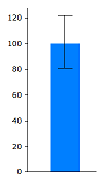
Error bars are widely used in science and engineering to show uncertainties in data.
Road casualties occur randomly, so numbers can rise and fall from year to year, just by chance.
Error bars (confidence intervals) can be used to show the size of this year-to-year random variation.
Such error bars on road casualty charts help to distinguish real changes in road risk from chance variation ("the signal from the noise").
There should be greater use of error bars (confidence intervals) by the DfT and others in presenting road casualty statistics.

Random variation in road casualty numbers

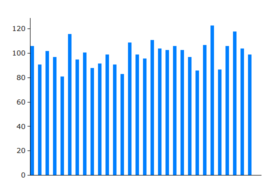
Random variation when the average rate is 100 events per year

Road casualties are generally random events. So they do not occur at regular intervals, and the number occurring in any period (e.g. a week, month or year) can change considerably even when road conditions have not changed.

The chart on the right indicates the size of random variation where an event occurs on average 100 times per year. Each bar represents one year, and the chart shows a typical pattern of variation over a period of 30 years when conditions have not changed. (It has been obtained by randomly distibuting 3000 event over the 30 years - the 3000 being the total of 100 events per year for 30 years).

The average number per year is 100, but the actual number varies from around 80 to around 120, just by chance. This random variation is larger than many people expect.

For events occurring at a lower frequency, the proportional random variation is even larger, while for events occurring at a higher frequency, the proportional random variation is less. This is illustrated by the next four charts which show typical patterns of random variation for situations where, respectively, on average 10, 100, 1000, and 10,000 events occur per year.

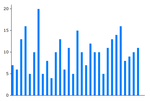Random variation when the average rate is 10 events per year	Random variation when the average rate is 100 events per year
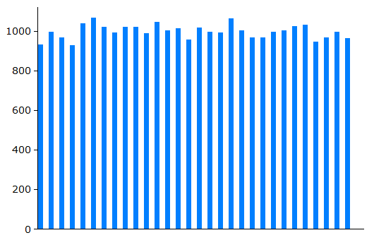Random variation when the average rate is 1000 events per year	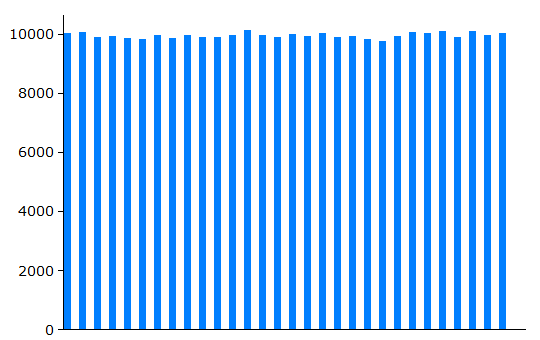Random variation when the average rate is 10,000 events per year

These four charts illustrate what many people understand intuitively - that there is greater reliability where observations are based on larger numbers.

Dangers of misinterpretation of road casualty statistics

This random variation in road casualty figures is a problem when it comes to responding to changes in figures.

For example, in June 2012, the DfT announced the following changes in reported cyclist casualties for 2011 compared to 2010 [1].

Cyclists killed:	-4%
Cyclists killed or seriously injured (KSI):	+15%

What is the right response to these figures? Have things become better for cyclists (fewer deaths) or worse (more serious injuries)? At first sight, it is hard to make sense of these apparently inconsistent findings. Should we look for some explanation for deaths and serious injuries going in opposite directions - perhaps invoking an increase in less experienced cyclists?

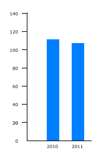Cyclists killed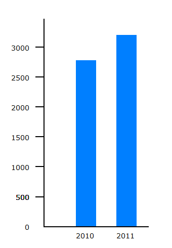

Cyclists KSI

Looking at the actual numbers and plotting charts gives the following charts.

The number of cyclists killed fell from 111 to 107. If we compare the Cyclists killed chart with the random variation chart for events occurring at a rate of 100 per year, it is apparent that the fall could easily be part of a pattern of random variation.

The number of reported cyclists KSI casualties rose from 2771 to 3192. Looking at the charts of random variation for events occurring at rates of 1000 and 10,000 per year, it seems that the rise could be outside the patterns of random variation seen.

To make sense of the changes recorded, we need to compare them with patterns of random variation. Otherwise there is a risk of jumping to false conclusions such as

assuming that recorded declines indicate that road safety measures are working, or
assuming that recorded rises indicate that road safety measures are not working, and so on.

The standard approach in statistics is to indicate random variation on charts via errors bars showing what are known as confidence intervals.

How confidence intervals are calculated

The standard approach is to consider how much random variation there is when conditions do not change, and calculate within what range most values will occur. The meaning of 'most values' is generally taken to be 95%. We can then use these calculations to produce a range of plausible values for the long term average when all we have is a single year's recorded number, and this range is termed a 95% confidence interval. This gives an indication of random year-to-year variation which can be used so that any changes from one year to another can be assessed as falling within random variation or as exceeding random variation.

There is an approximate formula that can be used as a rule of thumb for calculating 95% confidence intervals for random events (the technical terminology is events occurring as a Poisson variable):

Take the number of events recorded.
Take its square root.
Double this square root.
Take this (double the square root) away from the number recorded to give the lower end of the 95% confidence interval, and add this to the number recorded to give the upper end of the 95% confidence interval.

So supposing a number of 100 was recorded, taking the square root gives 10, doubling this gives 20, and the 95% confidence interval is from 100-20 to 100+20, i.e. from 80 to 120. This approximate formula works less well for values less than 100.

For road casualties, there is a complication that casualties do not occur entirely at random - there may be several people injured in a single collision, and very occasionally dozens. This increases the random variation in road casualty figures, but rarely to an appreciable extent.

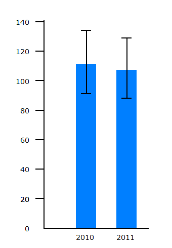Cyclists killed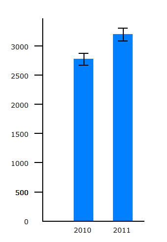

Cyclists KSI

Returning to the example of 2011 reported GB cyclist casualties, the charts on the right are the same as shown before but with 95% confidence intervals added.

It is clear that the fall in reported deaths is well within year-to-year random variation. So no conculsion can be drawn that this fall is part of a long term trend. If we want to look at long term trends in deaths, then we need to look a the figures for a longer period of time.

It is clear that the rise in reported cyclist KSIs is well outside year-to-year random variation, so some other explanation is needed.

Confidence intervals should be used more widely in road casualty statistics

Confidence intervals are widely used in many branches of statistics to show uncertainty in collected figures. For example, confidence intervals are widely used in medicine, and the International Committee of Medical Journal Editors has made recommendations for medical journal manuscripts that state

When possible, quantify findings and present them with appropriate indicators of measurement error or uncertainty (such as confidence intervals) [2].

Use of confidence intervals is discussed in detail in a recent article from the Washington State Department of Health[3]. The book by Altman et al provides tables and formulae[4].

Confidence intervals are currently little used in the presentation of road casualty statistics, and this can lead to errors of interpretation. The advantages of using confidence intervals should lead to their adoption into routine practice.

Random event simulator

This simulator was used to generate the charts of random variation on this web page. It uses random numbers to allocate the total number of events to the individual years at random.
As an example, try 100 events per year and 300 years.

References

[1]	DfT (June 2012). Reported road casualties Great Britain: main results 2011.https://www.gov.uk/government/publications/reported-road-casualties-great-britain-main-results-2011
[2]	International Committee of Medical Journal Editors (2013). Uniform Requirements for Manuscripts Submitted to Biomedical Journals: Manuscript Preparation and Submission. http://www.icmje.org/manuscript_1prepare.html
[3]	Washington State Department of Health (2012). Guidelines for Using Confidence Intervals for Public Health Assessment. www.doh.wa.gov/Portals/1/Documents/5500/ConfIntGuide.pdf
[4]	Statistics with Confidence 2nd Ed. (2000) Altman D, Machin D, Bryant T, and Gardner S. BMJ books. ISBN-10: 0727913751.